NTU教授Hung-yi Lee 老师22年的机器学习网课笔记，学习！！

Introduction of Machine Learning

Machine Learning = Looking for Function

Different Types of Functions

Regression (回归)：The function outputs a scalar value.
Classification (分类)：The function outputs a class labeld.

How to Find the Function

Function with UnKnown Parameters(参数)

$y=f(x)$
$y=w*x+b$
$y=w_1 x_1+w_2 x_2+…+w_n x_n+b$

Define Loss from Training Data.误差函数是自己定义的，也可能是负数。

Loss is a function of parameters.
Loss: how good a set of value is.
Label: the true value.
$L=\frac{1}{n}\sum_{i=1}^{n}(e_n)$
- e=$abs(y_{true}-y_{pred})$ L is mean absolute error(MAE) 标准差
- e=$\frac{1}{2}(y_{true}-y_{pred})^2$ L is mean squared error(MSE) 均方差
Error Surface: the surface of the loss function.根据参数的不同，loss的值不同，可以画出一个三维的图像，这个图像就是error surface

Minimize Loss by Optimizing Parameters.通过不断的调整参数，使得loss最小化

Gradient Descent（梯度下降法）: a method to minimize the loss function.
hyperparameters: 人为设定的参数，比如learning rate, number of iterations.学习率和迭代次数
$\alpha$ : learning rate
$w_{new}=w_{old}-\alpha\frac{\partial L}{\partial w}$
$\frac{\partial L}{\partial w}$: the gradient of the loss function.
Repeat the process until convergence.

Linear Model 线性模型

Model Bias (模型偏差): 对于不同的数据集，模型的预测值和真实值之间的差距。
Piecewise Linear Model (分段线性模型): 通过多个线性模型的组合，可以拟合非线性的数据。

import matplotlib.pyplot as plt


x1 = [0, 1, 2]
y1 = [0, 1, 2]

x2 = [2, 3, 4]
y2 = [2, 4, 6]  

x3 = [4, 5, 6]
y3 = [6, 7, 8]  


plt.plot(x1, y1, label='Segment 1')
plt.plot(x2, y2, label='Segment 2')
plt.plot(x3, y3, label='Segment 3')


plt.xlabel('x')
plt.ylabel('y')
plt.legend()


plt.show()

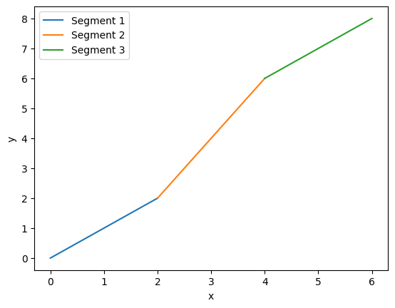
对于任何曲线，都可以用分段线性模型来拟合。

通过选取不同的函数类型，也可以更好地拟合数据。
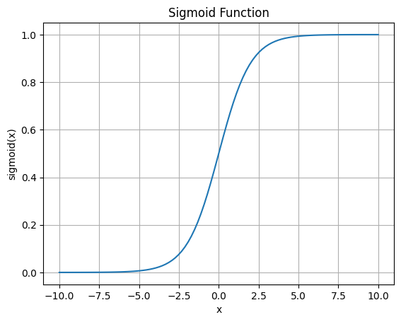
eg.对于z字型的曲线，可以使用soft sigmoid函数来拟合。

Soft sigmoid

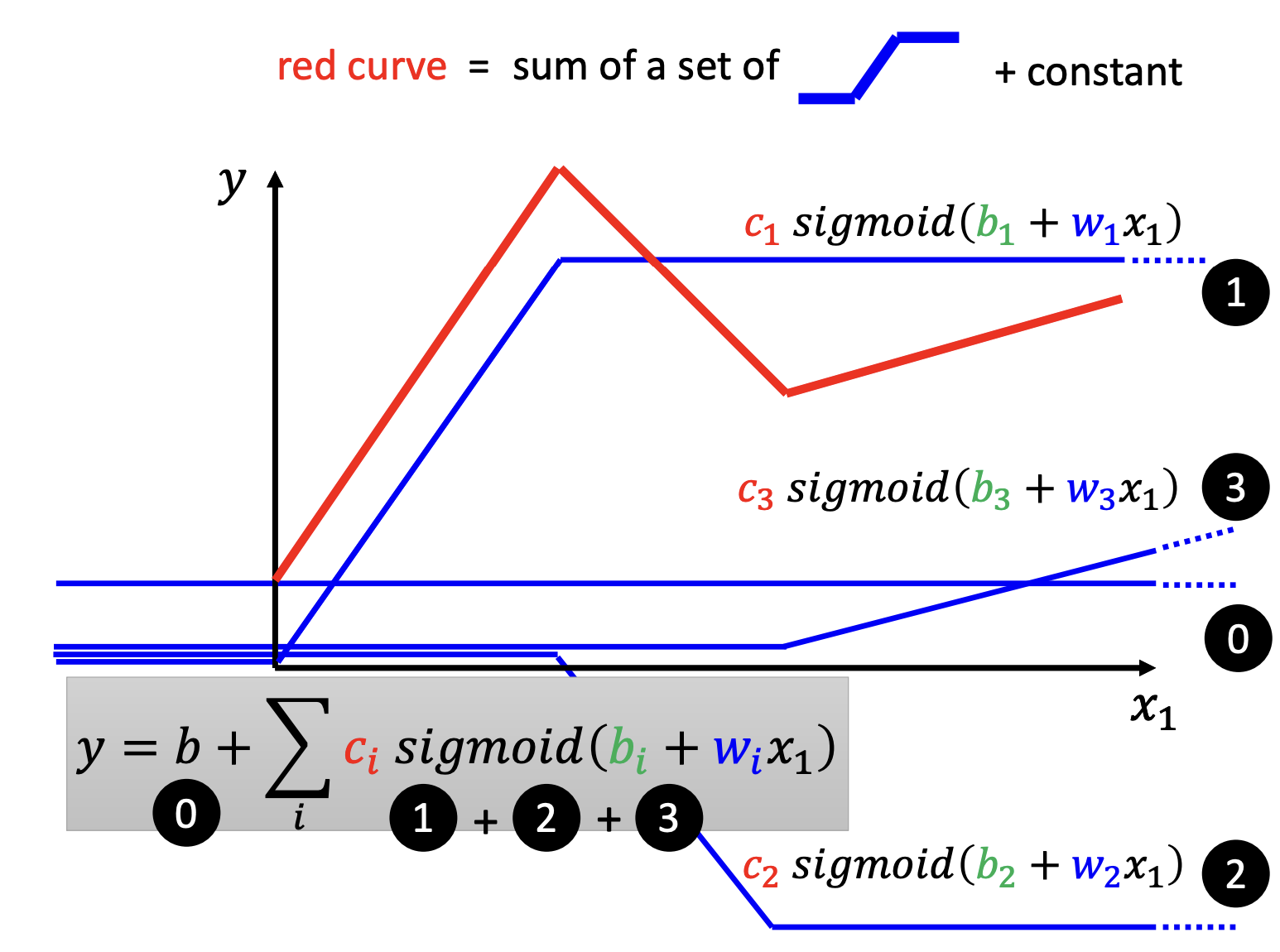
sigmoid function: $f(x)=\frac{1}{1+e^{-(b+wx_1)}}$

import numpy as np

import matplotlib.pyplot as plt

# Define the sigmoid function
def sigmoid(x):
    return 1 / (1 + np.exp(-x))

# Generate x values
x = np.linspace(-10, 10, 100)

# Calculate y values using the sigmoid function
y = sigmoid(x)

# Plot the sigmoid function
plt.plot(x, y)
plt.xlabel('x')
plt.ylabel('sigmoid(x)')
plt.title('Sigmoid Function')
plt.grid(True)
plt.show()

对于一个分段曲线，就可以这样拟合：

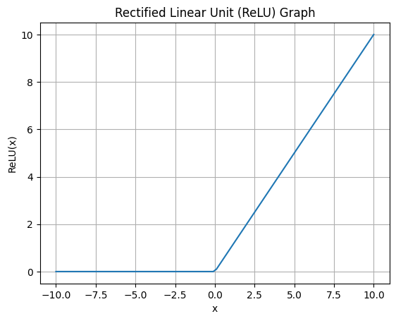
ReLU

Rectified Linear Unit(ReLU)线性整流函数:

$ c\ max(0,b+wx_1)$

import numpy as np

import matplotlib.pyplot as plt

# Define the ReLU function
def relu(x):
    return np.maximum(0, x)

# Generate x values
x = np.linspace(-10, 10, 100)

# Calculate y values using the ReLU function
y = relu(x)

# Plot the ReLU graph
plt.plot(x, y)
plt.xlabel('x')
plt.ylabel('ReLU(x)')
plt.title('Rectified Linear Unit (ReLU) Graph')
plt.grid(True)
plt.show()

Sigmoid 和 ReLU都可以叫做Activation Function激活函数,当然也有其他激活函数

Optimization of New Model:

对于每一个未知的参数，用$\theta$来表示，将所有的参数放在一个向量中，用 $\mathbf{\theta}$ 来表示。

$$
\mathbf{\theta} = \begin{bmatrix}
\theta _0 \\
\theta _1 \\
\theta _2 \\
\dots
\end{bmatrix}
$$

目标是求出使L最小的$\mathbf{\theta}$

$\mathbf{\theta}^* = argmin _\mathbf{\theta}\ L(\mathbf{\theta})$

(Randomly) pick initial values for $\mathbf{\theta} _0$.
Compute gradient
$$
\begin{aligned}
& g=\nabla L(\mathbf{\theta}^0) \\
& \mathbf{\theta}^1=\mathbf{\theta}^0-\alpha g
\end{aligned}
$$
Compute gradient
$$
\begin{aligned}
& g=\nabla L(\mathbf{\theta}^1) \\
& \mathbf{\theta}^2=\mathbf{\theta}^1-\alpha g
\end{aligned}
$$
Repeat until convergence.

update、epoch、layer

batch ：每次训练的数据量，相当于一个个包。
根据batch1，更新参数1，根据batch2，更新参数2，直到所有的数据都被训练过一遍。每一次更新所有参数，叫做一次update,所有的数据都被训练过一遍，叫做一个epoch。
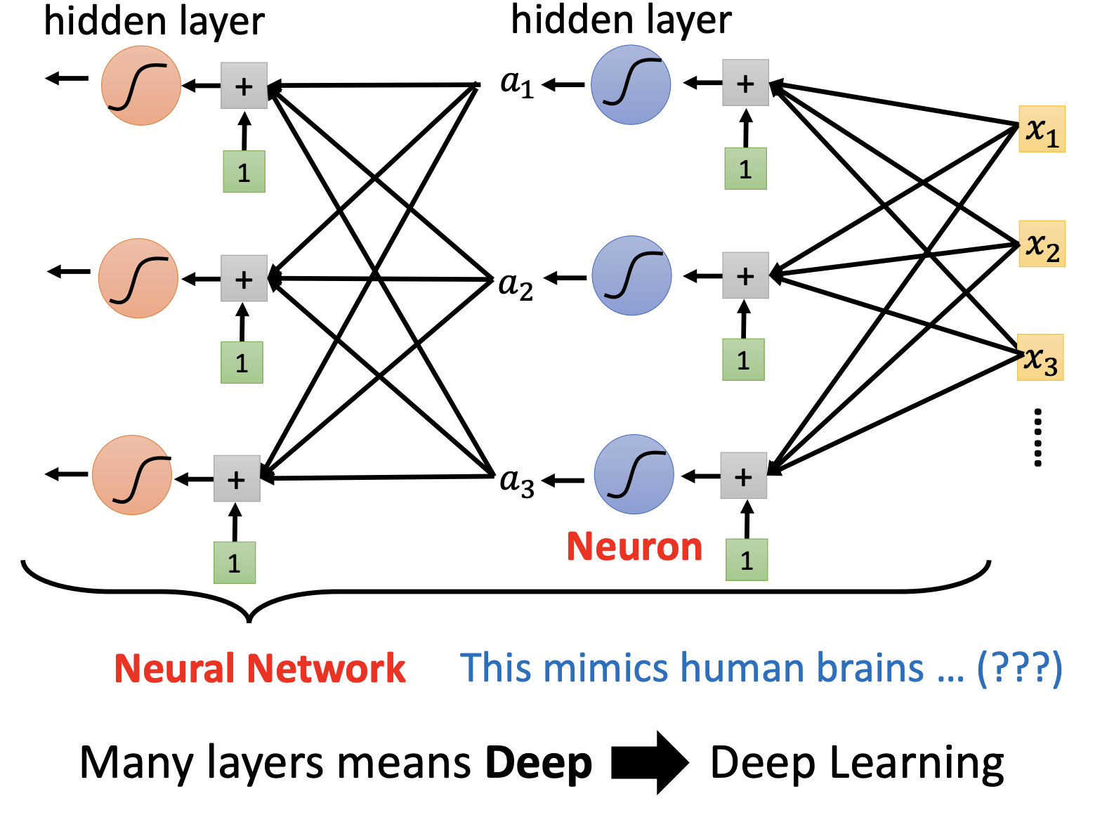
通过一次激活函数我们可以得到$\mathbf{a}=\sigma(\mathbf{b}+w\mathbf{x})$,我们将a视为下一个变量x’,进行下一次利用激活函数求出$\mathbf{a’}=\sigma(\mathbf{b’}+w\mathbf{x’})$，像这样子一次运算求得的一个参数就叫做一个Neuron(神经元)，每一排Neuron就叫做一个Later，所有Layer就是一个Neuron Network.

李宏毅老师ML 学习笔记【Introduction】